Bootstrapping

Caelan Bryan

Jenna Dufresne

Jamielee Jimenez Perez

Introduction

• Resampling is the process of creating new samples based on an observed sample to gather more information about either the sample or the population the sample came from.
• Resampling techniques like permutation tests, cross validation, and the jackknife have been prevalent in the statistics world for a while. Resampling can come in handy when it’s either impossible or unfeasible to retrieve a sample from the entire population.

Introduction (cont.)

• With resampling techniques you could verify the accuracy of the original sample, or make observations about the entire population of concert goers.
• All of the resampling techniques listed either have assumptions required for them to make meaningful results, fail at specific estimations, or produce errors during the process.
• The Bootstrap method was introduced to overcome some of the pitfalls of the jackknife resampling method.

What is the Bootstrap Method

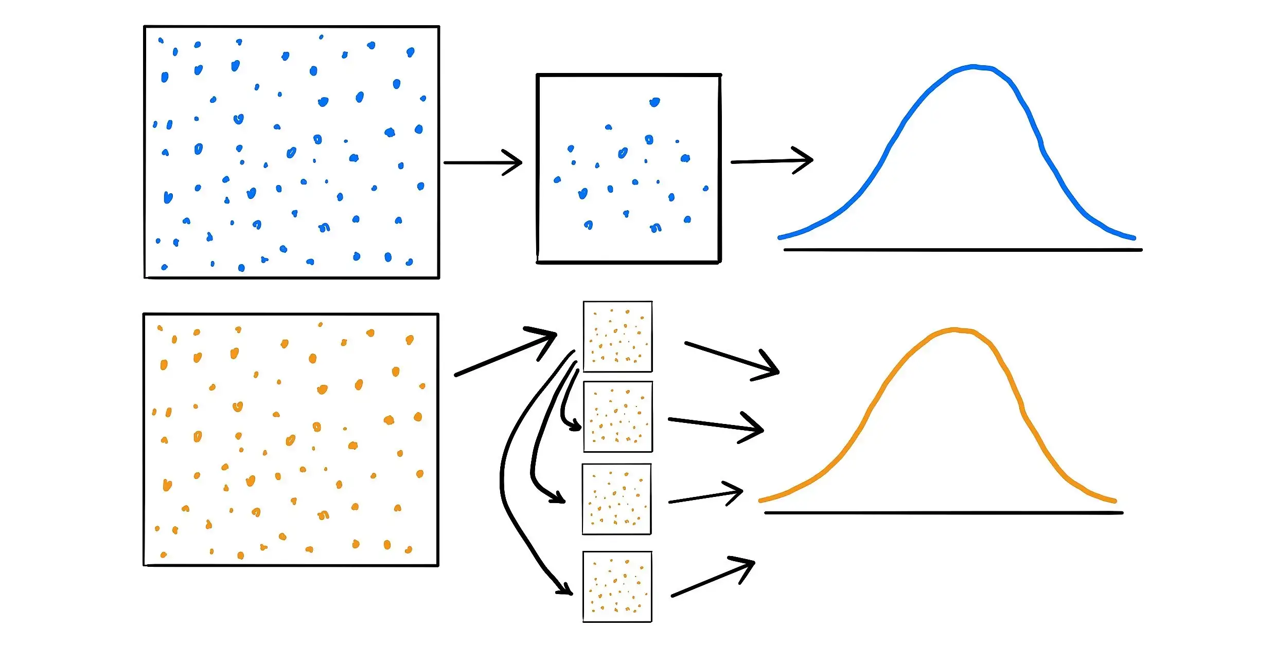
• Bootstrapping is the process of taking a sample and using it to create a new sample with replacement.
• Different version of the Bootstrap:
• Monte Carlo technique takes exact copies of the data from the original sample to place into the new sample (Hossain 2000)
• Bayesian Bootstrap adds weights to each observation before selecting the data for the new sample.
• This result in multiple different types of Bootstraps that can be used for different applications or to get around certain assumptions of another type of Bootstrap.

What is the Bootstrap Method (cont.)

figure 1 (Joseph 2020)

Assumptions and Shortcomings

• The Importance of Discussing Assumptions when Teaching Bootstrapping (Totty, Molyneux, and Fuentes 2021) states the largest assumption listed is that the distribution can be made approximately pivotal through shifting or studentization.
• Interesting result came out that if assumptions are broken when performing the Bootstrap method, it performs no better or worse then other methods whose assumptions are also broken.
• Performing Bootstrapping with broken assumptions can also lead to decreased performance of the method.

Continued

• One of the shortcomings of the Bootstrap method is that the results still rely on the original sample (Hossain 2000).
• if the original sample contains many outliers, then it most likely won’t produce an accurate representation of the population.
• Small sample sizes and data that does not follow a normal distribution has also been found to negatively impact the performance of Bootstrapping methods (Totty, Molyneux, and Fuentes 2021).

Application 1

• Bootstrapping has far reaching applications from finding a population mean to performing hypothesis testing. Initially, Efron introduced the Bootstrap method to estimate the sampling distribution, estimate the median, error rate estimation in discrimination analysis, Wilcoxon’s statistic, and regression models (B. Efron 1979).

Application 2

• In Nonparametric Estimates of Standard Error: The Jackknife, the Bootstrap, and Other Methods (Bradley Efron 1981). He introduces the concept of using the Bootstrap to estimate the standard error based on the data. While this is normally done using parametric modeling methods, in this article, it is being done with non-parametric methods, knowns as the Bootstrap.

Application 3

• Bootstrapping to create confidence intervals for certain statistics. Due to the nature of Bootstrapping, it creates results that make perfect sense to construct confidence intervals. Often, Bootstrapping implements confidence intervals around estimated parameter values (Puth, Neuhäuser, and Ruxton 2015). One example is using Bootstrapping to find the population mean of a specific feature based on the sample means. A few other similar applications are creating a confidence interval for the population mean and estimating the distribution of a sample mean (Hossain 2000).

Application 4

• Bootstrapping is in regression. In regression, the Bootstrap method can be used to perform validation on the model. In Bootstrapping with R to make generalized inference for regression model (Sillabutra et al. 2016) the authors used the Bootstrap method to resample thousands of times, fit a model to each new sample, and save the intercept and regression coefficient estimates. Confidence intervals can then be created to assess performance of a population regression model against the Bootstrap sample models.

Application 5

• The rise of statistical and mathematical programming languages and tools have greatly improved the state of Bootstrapping. Since Bootstrapping normally requires a large number of iterations to produce meaningful results, faster computers and tools have allowed statisticians to gain useful information. Software packages have been created for SAS, Stata (MD et al. 2005), and R (Sillabutra et al. 2016) that allow common Bootstrapping functionality to be used readily and easily.

Methods

1. Construct the sample probability distribution \(\hat{F}\), putting mass \(1/n\) at each point \(x_1, x_2, x_3, . . . , x_n\).
2. With \(\hat{F}\) fixed, draw a random sample of size \(n\) from \(\hat{F}\), say \(X_{i}^{*} = x_{i}^{*}\), \(X_{i}^{*} \sim _{ind}\hat{F}\) and call this the bootstrap sample.
3. Approximate the sampling distribution of \(R(X, \hat{F}\) by the bootstrap distribution of \(R^{*} = R(X^{*}, \hat{F})\).

Types of Bootstrap

1. Monte Carlo Case resampling
2. Exact Case resampling
3. Smooth Bootstrap

Monte Carlo Case resampling

In the Monte Carlo method, a new sample is created by randomly selecting values from the original sample using replacement to create a sample of the same size. Statistics can then be computed from this new sample. This process is then repeated many times to create an estimate of the population statistic. (B. Efron 1979)

Exact Case resampling

The exact version for Bootstrap case resampling is similar to the Monte Carlo method, except every possible enumeration of the initial sample is created. The downside to this method is since there are a total of \({2n - 1 \choose n} = \frac{(2n - 1)!}{n!(n - 1)!}\) possible samples, the process can be very intensive for large sample sizes. (Hossain 2000)

Smooth Bootstrap

• In the Smooth Bootstrap, a small amount of random noise is added to every resampled observation.
• This noise is zero-centered and usually normally distributed.
• Doing this means that the re-sampled data is not limited to just the data in the original sample, but rather to data points in close proximity to the original samples.

Other Types of Bootstrap

• Bayesian Bootstrap
  • Creates new sets by reweighting the initial data
• Parametric Bootstrap
  • Random observations are drawn from a fitted parametric model
• Poisson Bootstrap, Block Bootstrap, Wild Bootstrap, Gaussian Bootstrap

Figures

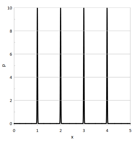
• Figure 2 shows an example of the simple bootstrap density function and Figure 3 shows an example of the smoothed density function provided by (Dwornicka, Goroshko, and Pietraszek 2019).

Figures (cont.)

Analysis and Results

Data and Visualization

• Causes of Death - Our World in Data (Chavez 2022)
  • 33 causes of death split by continent, region, country, and territory
  • Non-country entities removed
  • Execution and terrorism columns removed
  • Vatican and Liechtenstein are not included
• World Bank Population (2022)
  • Population for every year split by continent, region, country, and territory

Data and Visualization (cont.)

Name	Type
Entity	Nominal
Population	Discrete
Number_of_Deaths	Discrete
Deaths_CardiovascularDiseases	Nominal
Deaths_InterpersonalViolence	Discrete
Deaths_CardiovascularDiseasesRate	Continuous

Data and Visualization (cont.)

# Find cardiovascular disease death rate statistics
boot_means <- boot_data %>% summarize(mean_cardiovasculardiseasesrate = 
                                        mean(Deaths_CardiovascularDiseasesRate),
                                      sd_cardiovasculardiseasesrate = 
                                        sd(Deaths_CardiovascularDiseasesRate))

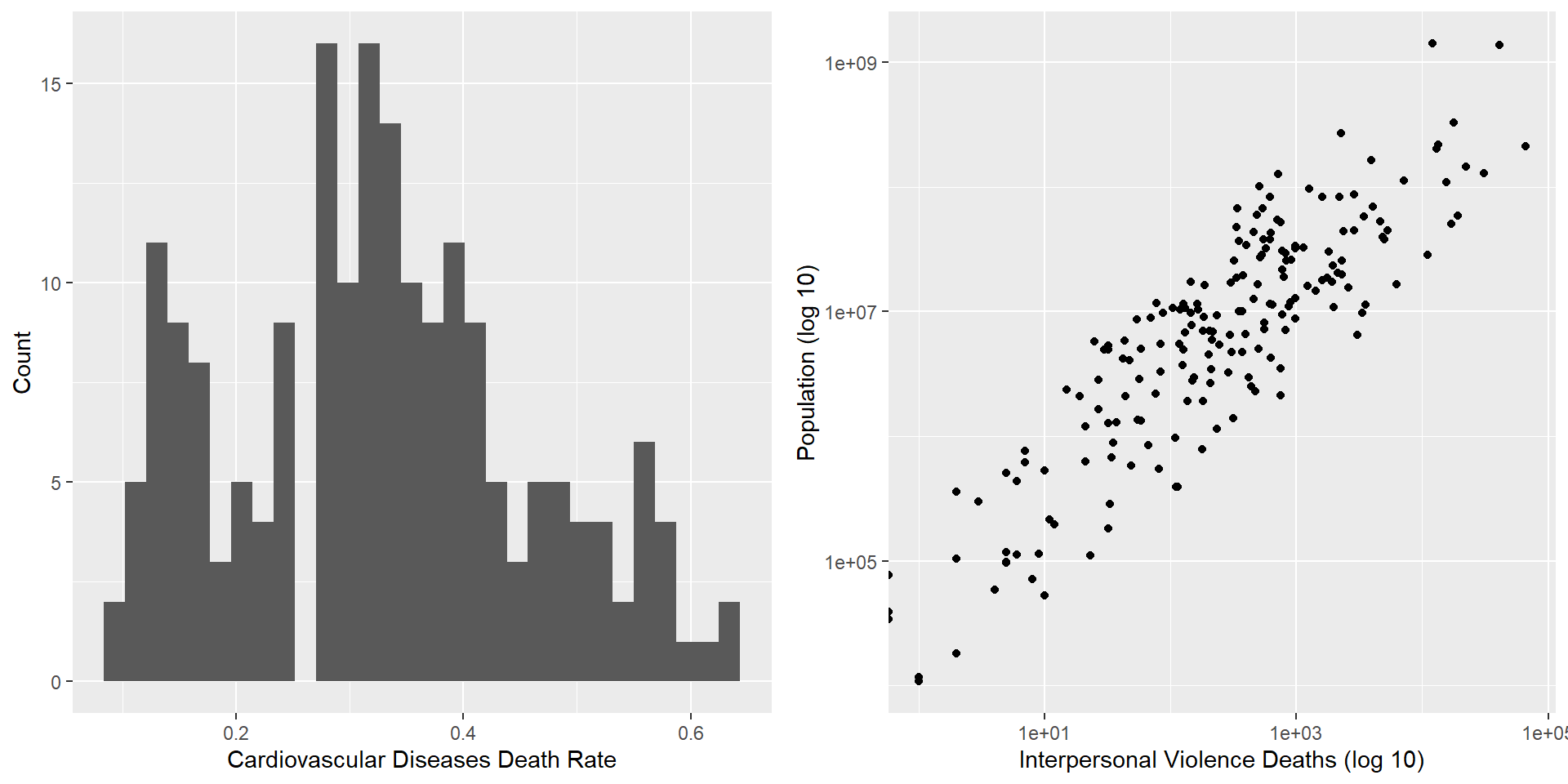
• Average rate of deaths caused by cardiovascular diseases is 32.73%

• Standard deviation of 13.09%

Data and Visualization (cont.)

# Create a histogram of the cardiovascular diseases death rate
cardioHistogram <- ggplot(boot_data, 
                          aes(x = Deaths_CardiovascularDiseasesRate)) +
                   xlab('Cardiovascular Diseases Death Rate') +
                   ylab('Count') +
                   geom_histogram()

# Plot the interpersonal violence death rate against population
violenceHistogram <- ggplot(boot_data, 
                            aes(x = Deaths_InterpersonalViolence, 
                                y = Population)) +
                     scale_x_log10() +
                     scale_y_log10() +
                     xlab('Interpersonal Violence Deaths (log 10)') +
                     ylab('Population (log 10)') +
                     geom_point() 

# Display plots side by side
grid.arrange(cardioHistogram, violenceHistogram, ncol = 2)

Data and Visualization (cont.)

Statistical Modeling

• Monte Carlo Method

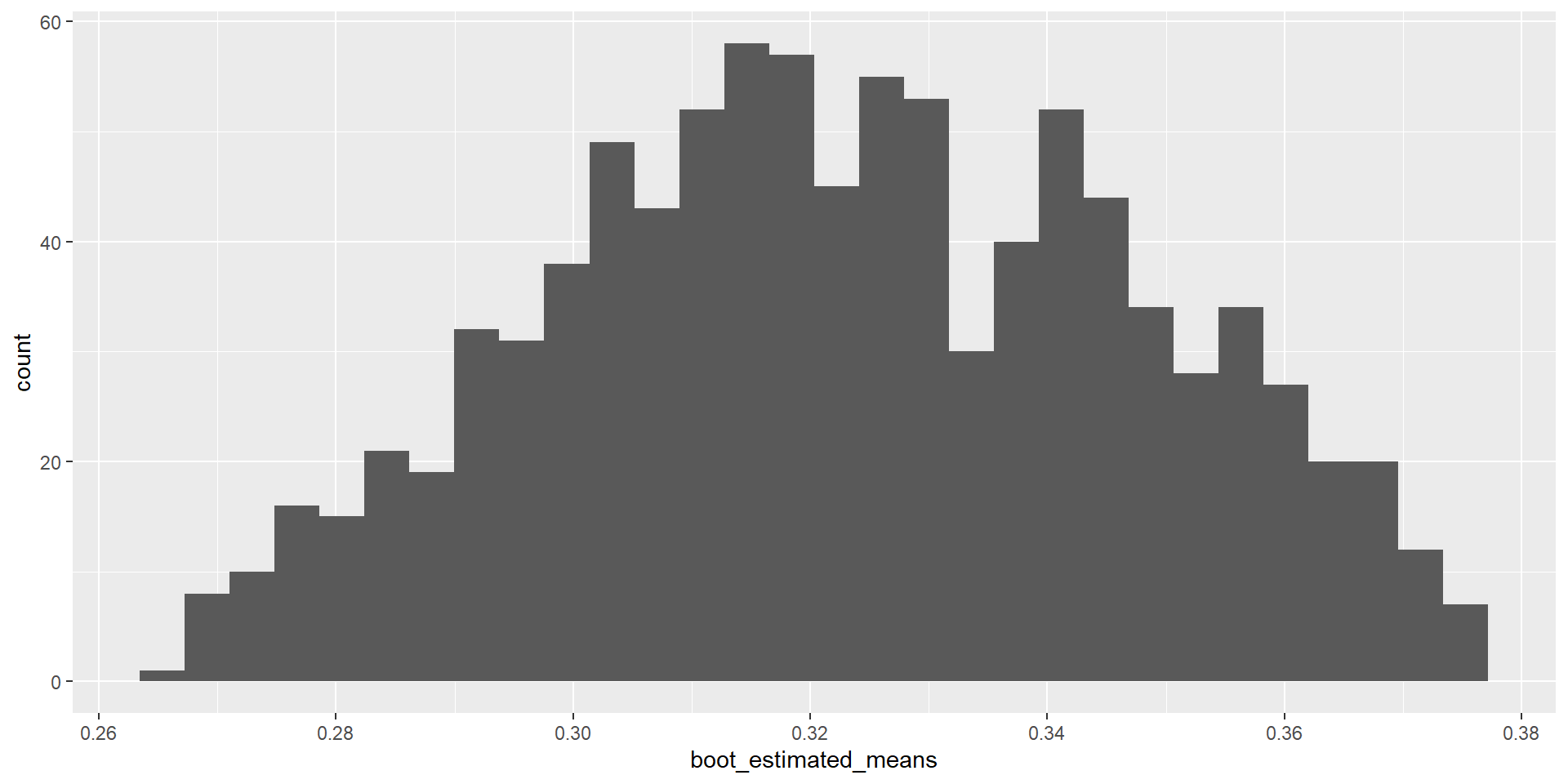
• 1,000 Bootstrap samples

• Estimating Population Mean and Standard Deviation

• Analyzing Regression Model Variability

• Sample size \(n = 20\)

# Create the initial sample
boot_initial_sample <- sample(1:nrow(boot_data), 20, replace = FALSE)

Population Mean and Standard Deviation

• Save mean and standard deviation

# Create vectors to store new sample means and standard deviations
boot_estimated_means <- rep()
boot_estimated_sds <- rep()
# Create 1,000 new samples and save the means and standard deviations
for (x in 1:1000) {
  boot_new_sample <- sample(boot_initial_sample, 20, replace = TRUE)
  boot_estimated_means <- append(boot_estimated_means,
                                 pull(
                                   summarize(
                                     boot_data[boot_new_sample,], 
                                     mean(Deaths_CardiovascularDiseasesRate))))
  boot_estimated_sds <- append(boot_estimated_sds, 
                               pull(
                                 summarize(
                                   boot_data[boot_new_sample,], 
                                   sd(Deaths_CardiovascularDiseasesRate))))
}

Population Mean and Standard Deviation (cont.)

• Trim top and bottom to find confidence interval

# Sort the estimated means from smallest to largest
boot_estimated_means <- sort(boot_estimated_means)
# Sort the estimated standard deviations from smallest to largest
boot_estimated_sds <- sort(boot_estimated_sds)
# Trim the top and bottom 2.5%
start = length(boot_estimated_means) * 0.025
end = length(boot_estimated_means) * 0.975
boot_estimated_means <- boot_estimated_means[start:end]
boot_estimated_sds <- boot_estimated_sds[start:end]

Population Mean and Standard Deviation (cont.)

• Select first and last values to find confidence intervals

• Compare against true population mean and standard deviation

• Estimated population mean

  • \(0.2658 < 0.3273 < 0.3758\)

• Estimated population standard deviation

  • \(0.0923 < 0.1309 < 0.1584\)

Population Mean and Standard Deviation (cont.)

# Display a histogram of the estimated means from the Bootstrap samples
ggplot() +
geom_histogram(aes(boot_estimated_means))

Regression Model Variability

• Save intercept and x1

# Create vectors to store new intercepts and regression parameters
boot_estimated_intercepts <- rep()
boot_estimated_regressionparameters <- rep()
# Create 1,000 new samples and save the intercepts and parameters
for (x in 1:1000) {
  boot_new_reg_sample <- sample(boot_initial_sample, 20, replace = TRUE)
  boot_new_lm <- lm(Deaths_InterpersonalViolence ~ Population,
                    boot_data[boot_new_reg_sample,])
  boot_estimated_intercepts <- append(boot_estimated_intercepts, 
                                      boot_new_lm$coefficients[1])
  boot_estimated_regressionparameters <- 
    append(boot_estimated_regressionparameters, 
           boot_new_lm$coefficients[2])
}

Regression Model Variability (cont.)

# Create population model
pop_lm <- lm(Deaths_InterpersonalViolence ~ Population, boot_data)
# Create initial sample model
sample_lm <- lm(Deaths_InterpersonalViolence ~ Population, 
                boot_data[boot_initial_sample,])
# Find Bootstrapping average values
boot_lm_intercept <- mean(boot_estimated_intercepts) 
boot_lm_x1 <- mean(boot_estimated_regressionparameters)

	Population	Sample	Bootstrap
(Intercept)	1183.7273	-1801.4852	-1500.0582
x	2.4^{-5}	1.74^{-4}	1.54^{-4}

Regression Model Variability (cont.)

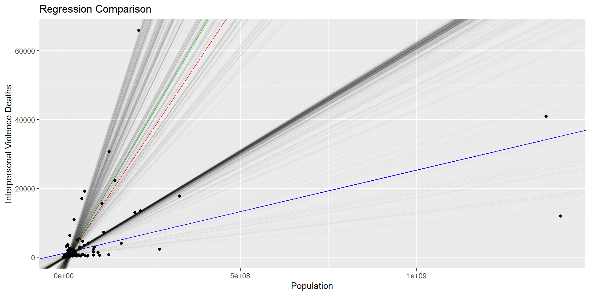
# Plot the data, population model, sample model, and final Bootstrap model 
# (average of all models)
final_plot <- ggplot(aes(x = Population, y = Deaths_InterpersonalViolence), 
                     data = boot_data) +
              geom_point() +
              geom_abline(intercept = coef(pop_lm)[1], 
                          slope = coef(pop_lm)[2], 
                          color= 'blue') +
              geom_abline(intercept = coef(sample_lm)[1], 
                          slope = coef(sample_lm)[2], 
                          color = 'green') +
              geom_abline(intercept = mean(boot_estimated_intercepts), 
                          slope = mean(boot_estimated_regressionparameters), 
                          color = 'red') +
              xlab('Population') + 
              ylab('Interpersonal Violence Deaths') +
              ggtitle('Regression Comparison') +
              labs(color = "Model")
# Add all Bootstrap models
for (x in 1:length(boot_estimated_intercepts)) {
  final_plot <- final_plot + 
                geom_abline(intercept = boot_estimated_intercepts[x], 
                            slope = boot_estimated_regressionparameters[x], 
                            alpha = 0.025)
}
# Display final plot
final_plot

Regression Model Variability (cont.)

Conclusion

In the first experiment, the population mean and standard deviation were estimated using the Bootstrap method and it was found that the confidence interval for both the mean and standard deviation fell within the confidence intervals and the population had a normal distribution.

In the second experiment, the simple linear regression model to estimate the number of deaths caused by interpersonal violence on the country population was analyzed for variability in the model. It was found that the Bootstrap model usually follows the sample model more closely than the full population model.

References

2022. https://data.worldbank.org/indicator/SP.POP.TOTL.

Chavez, Ivan. 2022. https://www.kaggle.com/datasets/ivanchvez/causes-of-death-our-world-in-data.

Dwornicka, Renata, Andrii Goroshko, and Jacek Pietraszek. 2019. “The Smoothed Bootstrap Fine-Tuning.” System Safety: Human - Technical Facility - Environment 1 (1): 716–23. https://doi.org/doi:10.2478/czoto-2019-0091.

Efron, B. 1979. “Bootstrap Methods: Another Look at the Jackknife.” The Annals of Statistics 7 (1): 1–26. http://www.jstor.org/stable/2958830.

Efron, Bradley. 1981. “Nonparametric Estimates of Standard Error: The Jackknife, the Bootstrap and Other Methods.” Biometrika 68 (3): 589–99. http://www.jstor.org/stable/2335441.

Hossain, Mohammad. 2000. “Bootstrapping – an Introduction and Its Applications in Statistics.” Bangladesh Journal of Scientific Research 18 (January): 75–88.

Joseph, Trist’n. 2020. “Bootstrapping Statistics. What It Is and Why It’s Used.” Medium. Towards Data Science. https://towardsdatascience.com/bootstrapping-statistics-what-it-is-and-why-its-used-e2fa29577307.

MD, MS, PhD MD, Jason Haukoos, and Roger Lewis. 2005. “Advanced Statistics: Bootstrapping Confidence Intervals for Statistics with ‘Difficult’ Distributions.” Academic Emergency Medicine 12 (April): 360–65. https://doi.org/10.1197/j.aem.2004.11.018.

Puth, Marie-Therese, Markus Neuhäuser, and Graeme D. Ruxton. 2015. “On the Variety of Methods for Calculating Confidence Intervals by Bootstrapping.” Journal of Animal Ecology 84 (4): 892–97. https://doi.org/https://doi.org/10.1111/1365-2656.12382.

Sillabutra, Jutatip, Prasong Kitidamrongsuk, Chukiat Viwatwongkasem, Chareena Ujeh, Siam Sae-tang, and Khanokporn Donjdee. 2016. “Bootstrapping with r to Make Generalized Inference for Regression Model.” Procedia Computer Science 86: 228–31. https://doi.org/https://doi.org/10.1016/j.procs.2016.05.103.

Totty, Njesa, James Molyneux, and Claudio Fuentes. 2021. “The Importance of Discussing Assumptions When Teaching Bootstrapping.” arXiv. https://doi.org/10.48550/ARXIV.2112.07737.